pacman::p_load(igraph, tidygraph, ggraph,
               visNetwork, lubridate, clock,
tidyverse, graphlayouts)inclass08
GAStech_nodes <- read_csv("data/GAStech_email_node.csv")Rows: 54 Columns: 4
── Column specification ────────────────────────────────────────────────────────
Delimiter: ","
chr (3): label, Department, Title
dbl (1): id
ℹ Use `spec()` to retrieve the full column specification for this data.
ℹ Specify the column types or set `show_col_types = FALSE` to quiet this message.GAStech_edges <- read_csv("data/GAStech_email_edge-v2.csv")Rows: 9063 Columns: 8
── Column specification ────────────────────────────────────────────────────────
Delimiter: ","
chr (5): SentDate, Subject, MainSubject, sourceLabel, targetLabel
dbl (2): source, target
time (1): SentTime
ℹ Use `spec()` to retrieve the full column specification for this data.
ℹ Specify the column types or set `show_col_types = FALSE` to quiet this message.glimpse(GAStech_edges)Rows: 9,063
Columns: 8
$ source <dbl> 43, 43, 44, 44, 44, 44, 44, 44, 44, 44, 44, 44, 26, 26, 26…
$ target <dbl> 41, 40, 51, 52, 53, 45, 44, 46, 48, 49, 47, 54, 27, 28, 29…
$ SentDate <chr> "6/1/2014", "6/1/2014", "6/1/2014", "6/1/2014", "6/1/2014"…
$ SentTime <time> 08:39:00, 08:39:00, 08:58:00, 08:58:00, 08:58:00, 08:58:0…
$ Subject <chr> "GT-SeismicProcessorPro Bug Report", "GT-SeismicProcessorP…
$ MainSubject <chr> "Work related", "Work related", "Work related", "Work rela…
$ sourceLabel <chr> "Sven.Flecha", "Sven.Flecha", "Kanon.Herrero", "Kanon.Herr…
$ targetLabel <chr> "Isak.Baza", "Lucas.Alcazar", "Felix.Resumir", "Hideki.Coc…Data Wrangling
GAStech_edges <- GAStech_edges %>%
  mutate(SendDate = dmy(SentDate))%>%
  mutate(Weekday = wday(SentDate,
                        label = TRUE,
                        abbr =FALSE))
GAStech_edges_aggregated <- GAStech_edges %>%
filter(MainSubject == "Work related") %>%
group_by(source, target, Weekday) %>%
summarise(Weight = n()) %>%
filter(source!=target) %>%
filter(Weight > 1) %>%
ungroup()`summarise()` has grouped output by 'source', 'target'. You can override using
the `.groups` argument.GAStech_graph <- tbl_graph(nodes = GAStech_nodes,
edges = GAStech_edges_aggregated,
directed = TRUE)
GAStech_graph# A tbl_graph: 54 nodes and 1372 edges
#
# A directed multigraph with 1 component
#
# Node Data: 54 × 4 (active)
id label Department Title
<dbl> <chr> <chr> <chr>
1 1 Mat.Bramar Administration Assistant to CEO
2 2 Anda.Ribera Administration Assistant to CFO
3 3 Rachel.Pantanal Administration Assistant to CIO
4 4 Linda.Lagos Administration Assistant to COO
5 5 Ruscella.Mies.Haber Administration Assistant to Engineering Group Manag…
6 6 Carla.Forluniau Administration Assistant to IT Group Manager
# … with 48 more rows
#
# Edge Data: 1,372 × 4
from to Weekday Weight
<int> <int> <ord> <int>
1 1 2 Sunday 5
2 1 2 Monday 2
3 1 2 Tuesday 3
# … with 1,369 more rowsGAStech_graph %>%
activate(edges) %>%
arrange(desc(Weight))# A tbl_graph: 54 nodes and 1372 edges
#
# A directed multigraph with 1 component
#
# Edge Data: 1,372 × 4 (active)
from to Weekday Weight
<int> <int> <ord> <int>
1 40 41 Saturday 13
2 41 43 Monday 11
3 35 31 Tuesday 10
4 40 41 Monday 10
5 40 43 Monday 10
6 36 32 Sunday 9
# … with 1,366 more rows
#
# Node Data: 54 × 4
id label Department Title
<dbl> <chr> <chr> <chr>
1 1 Mat.Bramar Administration Assistant to CEO
2 2 Anda.Ribera Administration Assistant to CFO
3 3 Rachel.Pantanal Administration Assistant to CIO
# … with 51 more rowsPlotting a basic network graph
ggraph(GAStech_graph) +
  geom_edge_link() +
  geom_node_point()
Using "stress" as default layoutWarning: Using the `size` aesthetic in this geom was deprecated in ggplot2 3.4.0.
ℹ Please use `linewidth` in the `default_aes` field and elsewhere instead.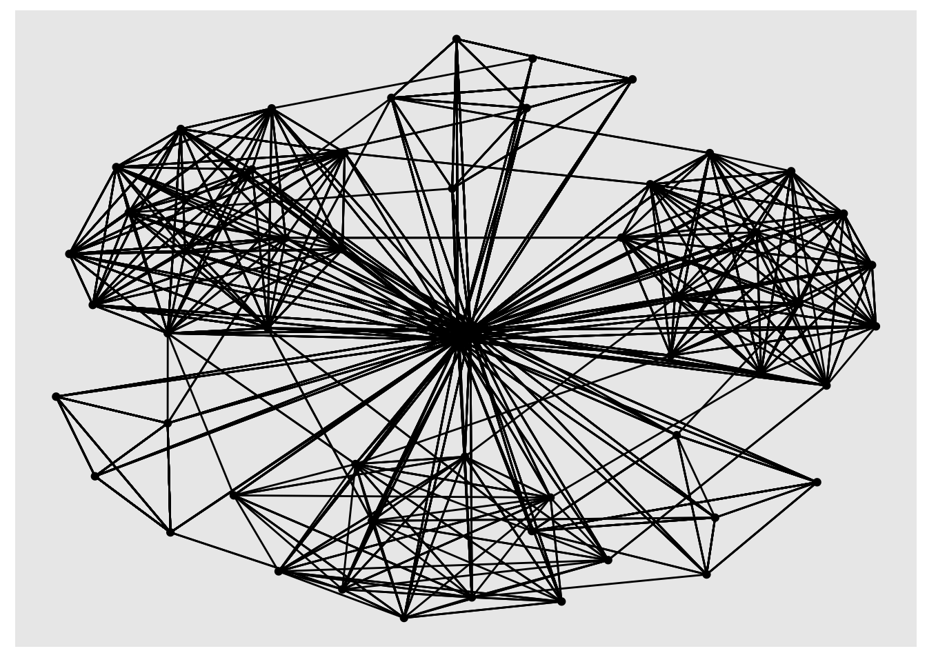
Changing the default network graph theme
g <- ggraph(GAStech_graph) +
  geom_edge_link(aes()) +
  geom_node_point(aes())
Using "stress" as default layoutg + theme_graph()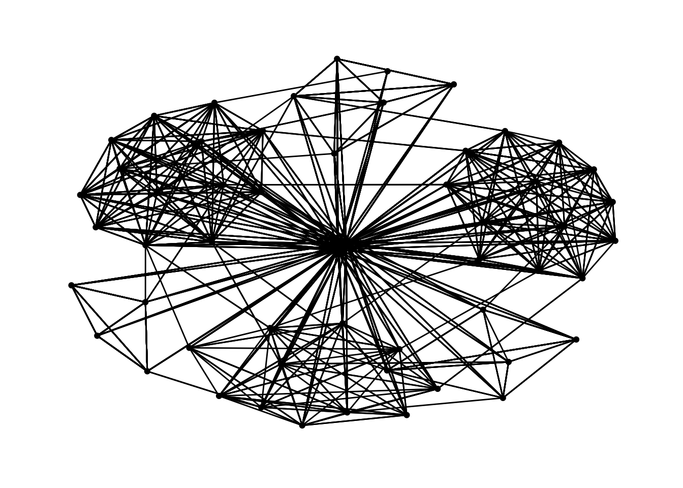
Changing the coloring of the plot
g <- ggraph(GAStech_graph) +
  geom_edge_link(aes(colour = 'grey50')) +
  geom_node_point(aes(colour = 'grey40'))
Using "stress" as default layoutg + theme_graph(background = 'grey10',
text_colour = 'white')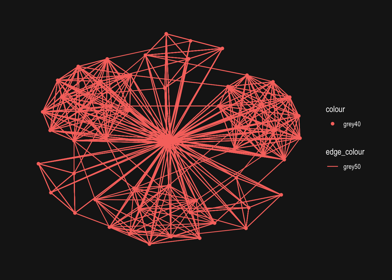
Fruchterman and Reingold layout
g <- ggraph(GAStech_graph,
            layout = "fr") +
  geom_edge_link(aes()) +
  geom_node_point(aes())

g + theme_graph()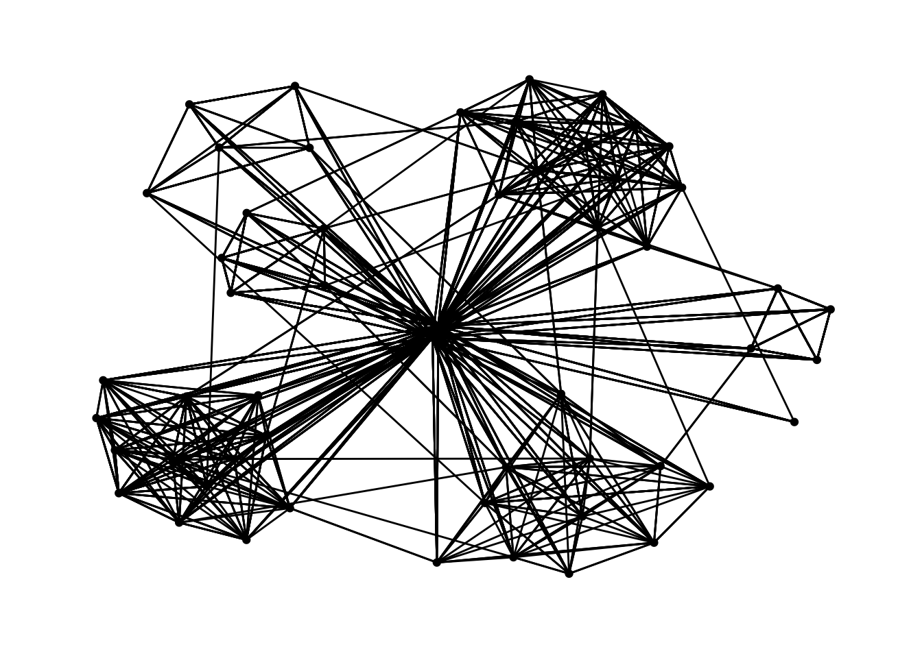
g <- ggraph(GAStech_graph,
            layout = "nicely") +
  geom_edge_link(aes()) +
  geom_node_point(aes(colour = Department,
                      size = 3))

g + theme_graph()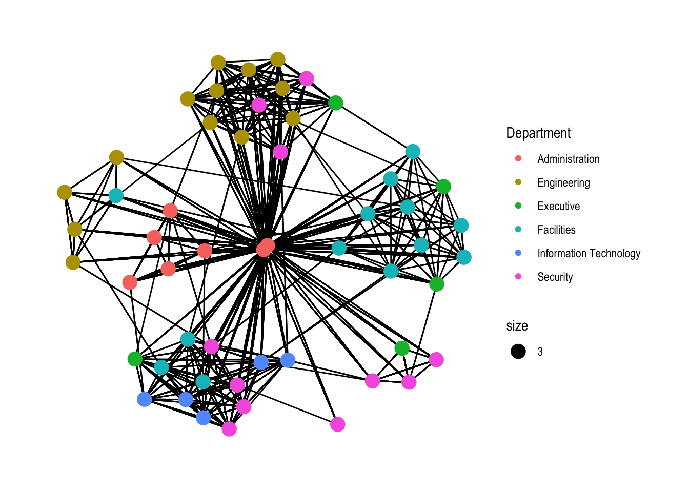
Modifying edges
g <- ggraph(GAStech_graph,
            layout = "nicely") +
  geom_edge_link(aes(width=Weight),
                 alpha=0.2) +
  scale_edge_width(range = c(0.1, 5)) +
  geom_node_point(aes(colour = Department),
                  size = 3)

g + theme_graph()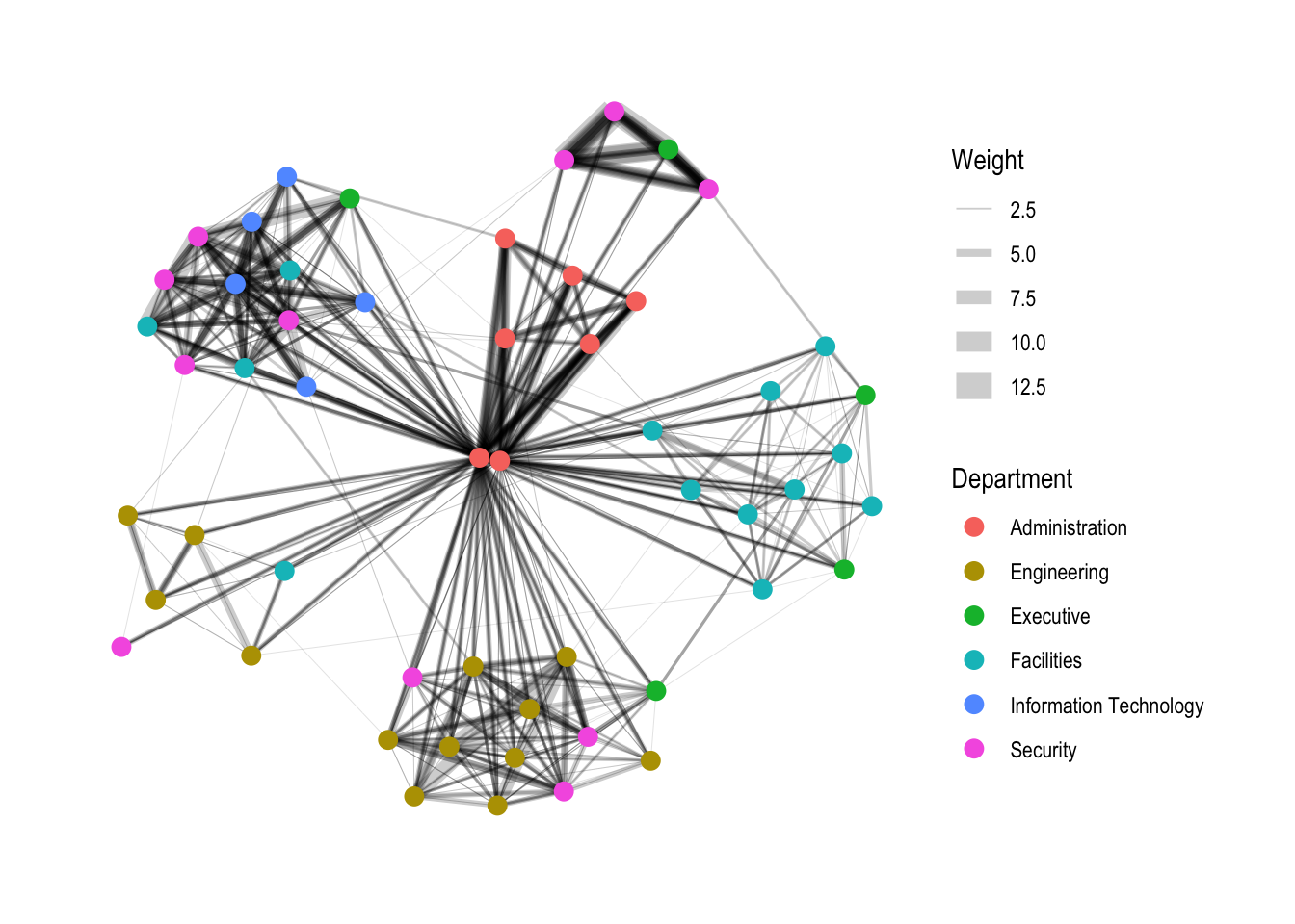
Creating facet graphs
Working with facet_edges()
set_graph_style()

g <- ggraph(GAStech_graph,
            layout = "nicely") +
  geom_edge_link(aes(width=Weight),
                 alpha=0.2) +
  scale_edge_width(range = c(0.1, 5)) +
  geom_node_point(aes(colour = Department),
                  size = 2)

g + facet_edges(~Weekday)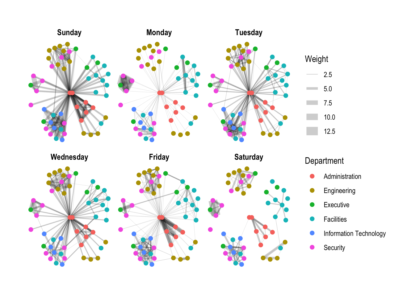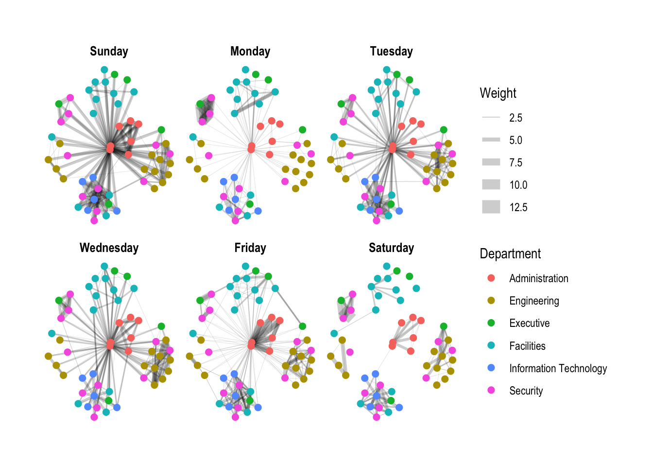
A framed facet graph
set_graph_style()

g <- ggraph(GAStech_graph,
            layout = "nicely") +
  geom_edge_link(aes(width=Weight),
                 alpha=0.2) +
  scale_edge_width(range = c(0.1, 5)) +
  geom_node_point(aes(colour = Department),
                  size = 2)

g + facet_edges(~Weekday) +
  th_foreground(foreground = "grey80",
                border = TRUE) +
  theme(legend.position = 'bottom')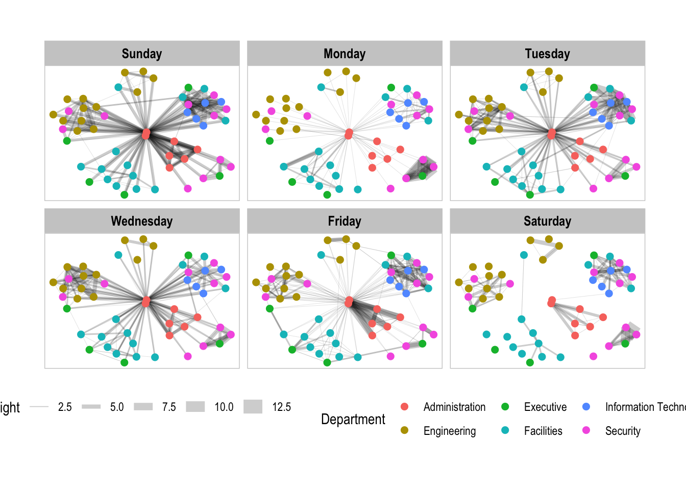
Working with facet_nodes()
set_graph_style()

g <- ggraph(GAStech_graph,
            layout = "nicely") +
  geom_edge_link(aes(width=Weight),
                 alpha=0.2) +
  scale_edge_width(range = c(0.1, 5)) +
  geom_node_point(aes(colour = Department),
                  size = 2)

g + facet_nodes(~Department)+
  th_foreground(foreground = "grey80",
                border = TRUE) +
  theme(legend.position = 'bottom')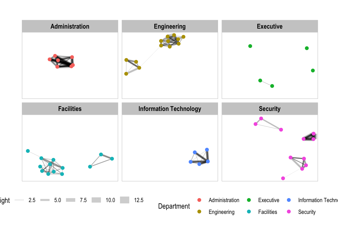
Network Metrics Analysis
g <- GAStech_graph %>%
  mutate(betweenness_centrality = centrality_betweenness()) %>%
  ggraph(layout = "fr") +
  geom_edge_link(aes(width=Weight),
                 alpha=0.2) +
  scale_edge_width(range = c(0.1, 5)) +
  geom_node_point(aes(colour = Department,
            size=betweenness_centrality))
g + theme_graph()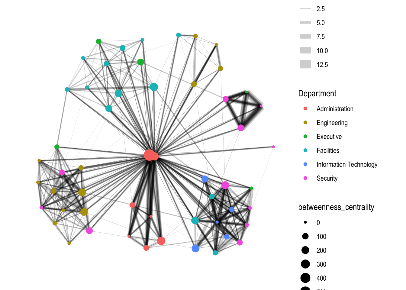
Visualising network metrics
g <- GAStech_graph %>%
  ggraph(layout = "fr") +
  geom_edge_link(aes(width=Weight),
                 alpha=0.2) +
  scale_edge_width(range = c(0.1, 5)) +
  geom_node_point(aes(colour = Department,
                      size = centrality_betweenness()))
g + theme_graph()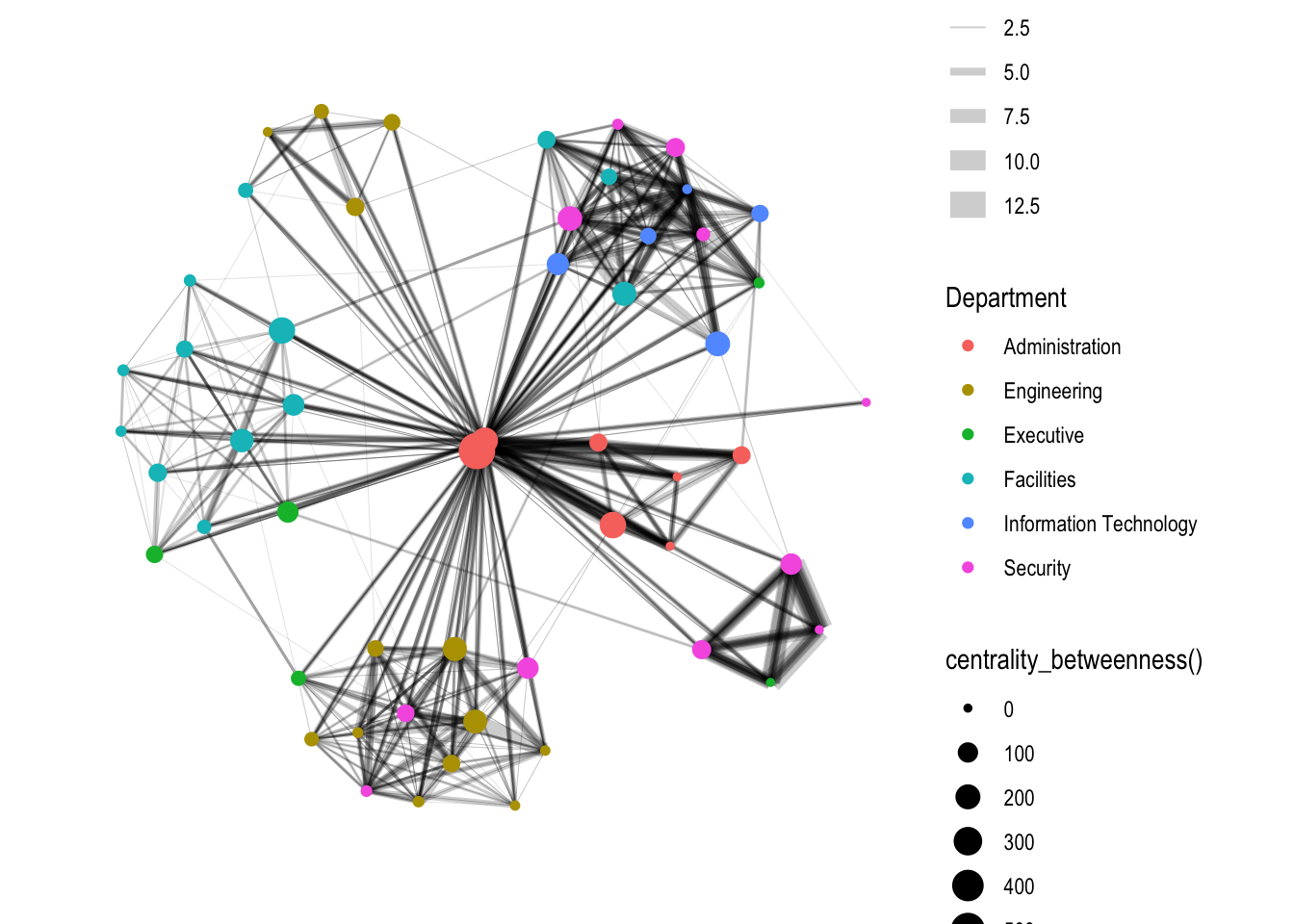
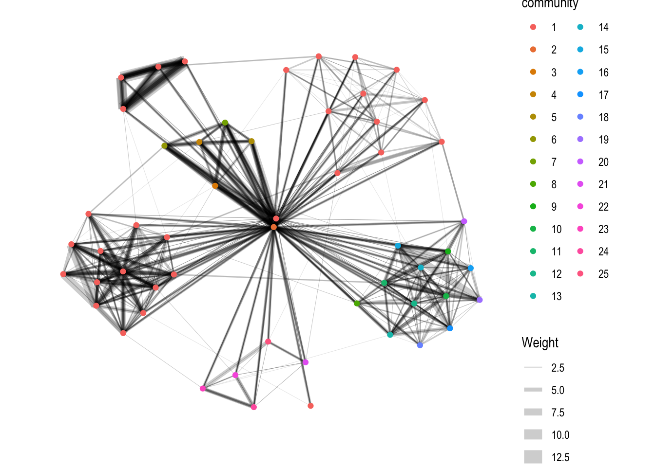
Visualising Community
g <- GAStech_graph %>%
  mutate(community = as.factor(group_edge_betweenness(weights = Weight, directed = TRUE))) %>%
  ggraph(layout = "fr") +
  geom_edge_link(aes(width=Weight),
                 alpha=0.2) +
  scale_edge_width(range = c(0.1, 5)) +
  geom_node_point(aes(colour = community))
Warning: There were 2 warnings in `mutate()`.
The first warning was:
ℹ In argument: `community = as.factor(group_edge_betweenness(weights = Weight,
directed = TRUE))`.
Caused by warning in `cluster_edge_betweenness()`:
! At core/community/edge_betweenness.c:493 : Membership vector will be selected based on the highest modularity score.
ℹ Run `dplyr::last_dplyr_warnings()` to see the 1 remaining warning.g + theme_graph()